Vignette: Simulation studies with `ValidationExplorer`

Abstract

Our vignette demonstrates the use of the ValidationExplorer package to conduct statistical simulation studies that can aid in the design phase of bioacoustic studies. In particular, our package facilitates exploration of the costs and inferential properties (e.g., coverage and interval widths) of alternative validation designs in the context of the count detection model framework. Our functions allow the user to specify a suite of candidate validation designs using either a stratified sampling procedure or a fixed-effort design type. An example of the former is provided in the manuscript entitled ‘ValidationExplorer: Streamlined simulations to inform bioacoustic study design in the presence of misclassification’, which was submitted to the Journal of Data Science. In this vignette, we provide further details not covered in the manuscript and an additional example of data simulation, model fitting, and visualization of simulation results when using a fixed-effort design type. Our demonstration here is intended to aid researchers and others to tailor a validation design that provides useful inference while also ensuring that the level of effort meets cost constraints.

Disclaimer: This draft manuscript is distributed solely for the purposes of scientific peer review. Its content is deliberative and pre-decisional, so it must not be disclosed or released by reviewers. Because the manuscript has not yet been approved for publication by the U.S. Geological Survey (USGS), it does not represent any official USGS funding or policy. Any use of trade, firm, or product names is for descriptive purposes only and does not imply endorsement by the U.S. Government.

Introduction

Automated recording units (ARUs) provide one of the main data sources for many contemporary ecological studies that aim to provide inference about status and trends for assemblages of species (Loeb et al. 2015). As described in the manuscript “ValidationExplorer: Streamlined simulations to inform bioacoustic study design in the presence of misclassification,” substantial practical interest lies in identifying cost-effective validation designs that will allow a study to obtain its measurable objectives. We believe that statistical simulation studies are a valuable tool for informing study design – including the validation step – prior to gathering ARU data, and it is our goal for ValidationExplorer to provide those tools in an approachable package.

This vignette aids exploration of possible validation designs within a count-detection framework using the ValidationExplorer package. As described in the main text, a validation design is composed of two parts: a random mechanism for selecting observations to be manually reviewed by experts (“validated”), and a percentage or proportion that controls the number of validated recordings. We refer to the random mechanism as the design type and the proportion as the level of validation effort (LOVE). In the following section we consider five possible LOVEs and show an example of a fixed effort design.

We emphasize that results from any simulation study – including those produced using the ValidationExplorer package – are conditional on the settings and assumptions of the study. In the case of the count-detection model framework that is implemented in ValidationExplorer, the assumptions are

The occurrence of species within a site are independent; the presence of one species carries no information about the presence or absence of another.
For any one species, its occurrence at one location is independent of its occurrence at any other location (independence across sites).
Visits to a site (i.e., detector nights) are independent.
Recordings within the same site-visit are independent.
Each recording is assigned a single species autoID.
Validation of one recording does not influence the probability that another will be validated.
At sites where at least one species is present, the count of recordings generated by each species per night is a Poisson random variable.
All species in the assemblage can co-occur and are capable of being confused (no structural zeros in the classification matrix).
The configuration of visits to sites is balanced. Note that this is not required to use our method but it is assumed in the simulation studies. For example, the data used by Oram et al. (in submission) had a varying number of detector nights at each site. To model these data, Oram et al. (in submission) made the additional assumption that the number of visits to a site is independent of the presence/absence and expected relative activity of species there. That is, locations where detectors were deployed for more nights were not more or less likely than other sites to be occupied by species of interest and were not more or less likely than other sites to have high levels of activity.
The fitted model is the same as the model that generated the data.

Under these assumptions, we outline the step-by-step use of ValidationExplorer in the following section.

Conducting a simulation study with a fixed effort design type

What is a fixed effort design?

In this section, we assume a fixed-effort design type, under which $x\%$ of recordings obtained from each visit to a site are validated by experts. The level of validation effort is controlled by the value of $x.$ We begin the process of simulating under this design by defining the real-world objectives and constraints we anticipate.

Step 0: Define measurable objectives and constraints

The first step – before opening R and loading ValidationExplorer – is to identify and write down the set of measurable objectives that the data will be used for. Suppose that, for this example, the measurable objectives and cost constraints are as follows:

The measurable objective is to estimate relative activity parameters (denoted as $\lambda_k$ ) for each species with 95% coverage and expected posterior interval width less than 3 calls per night.
The monitoring program can pay their expert bat biologists to validate at most 4000 recordings. We make the assumption that all recordings are approximately the same cost to validate (i.e., rare species autoIDs are not necessarily more expensive or time consuming than extremely common ones).

Suppose further that we have six species of interest that co-occur. The existing prior knowledge (perhaps from another study) about the relative activity rates and occurrence probabilities for each species are summarized in the following table:

Prior knowledge of relative activity rates and occurrence probabilities for the six bat species of interest. These values will be used to simulate data.
Species	$\psi$	$\lambda$
Eptesicus fuscus (EPFU)	0.63	5.9
Lasiurus cinereus (LACI)	0.61	4.2
Lasionycteris noctivagans (LANO)	0.85	14.3
Myotis californicus (MYCA)	0.70	6.2
Myotis ciliolabrum (MYCI)	0.24	11.9
Myotis evotis (MYEV)	0.70	2.4

Step 1: Installing and loading required packages

Once measurable objectives and constraints are clearly defined, the next step is to load the required packages. For first time users, it may be necessary to install a number of dependencies, as shown by Table 1 in the manuscript. If you need to install a dependency or update the version, run the following, with your_package_name_here replaced by the name of the package:

install.packages("your_package_name_here")

After installing the necessary packages, load these libraries by calling

library(tidyverse)
library(nimble)
library(coda)
library(rstan)
library(parallel)
library(here)

Finally, install and load ValidationExplorer by running

# Install development version
devtools::install_github(repo = "j-oram/ValidationExplorer")

# Load once installed
library(ValidationExplorer)

Step 2: Simulate data

The first step in a simulation study is to simulate data under each of the candidate validation designs, which is accomplished with the simulate_validatedData function in ValidationExplorer. We begin by assigning values for the number of sites, visits, and species, as well as the parameter values shown above, which are existing estimates obtained by Stratton et al. (2022):

# Set the number of sites, species and visits
nsites <- 30
nspecies <- 6
nvisits <- 4

psi <- c(0.6331, 0.6122, 0.8490, 0.6972, 0.2365, 0.7036)
lambda <- c(5.9347, 4.1603, 14.2532, 6.1985, 11.8649, 2.4050)

Note that by running multiple simulation studies with varying numbers of sites and balanced visits, ValidationExplorer allows users to investigate all elements of the study design prior to data collection. In addition to specifying the numnber of sites and visits and parameter values, simulate_validatedData requires that the user supply misclassification probabilities in the form of a matrix, subject to the constraint that rows in the matrix sum to one. An easy way to simulate a matrix of probabilities that meet these criteria is to leverage the rdirch function from the nimble package:

# Simulate a hypothetical confusion matrix 
set.seed(10092024) 
Theta <- t(apply(diag(29, nspecies) + 1, 1, function(x) {nimble::rdirch(alpha = x)}))

Note that the above definition of Theta places high values on the diagonal of the matrix, corresponding to a high probability of correct classification. To lower the diagonal values, change the specification of diag(29, nspecies) to a smaller value. For example:

another_Theta <- t(apply(diag(5, nspecies) + 1, 1, function(x) {
    nimble::rdirch(alpha = x)
  }))

another_Theta has lower values on the diagonal, and greater off-diagonal values (i.e., higher probability of misclassification). If you have specific values you would like to use for the assumed classification probabilities (e.g., from an experiment), these can be supplied manually:

manual_Theta <- matrix(c(0.9, 0.05, 0.01, 0.01, 0.02, 0.01, 
                       0.01, 0.7, 0.21, 0.05, 0.02, 0.01,  
                       0.01, 0.01, 0.95, 0.01, 0.01, 0.01,
                       0.05, 0.05, 0.03, 0.82, 0.04, 0.01,
                       0.01, 0.015,  0.005,  0.005, 0.95, 0.015,
                       0.003, 0.007, 0.1, 0.04, 0.06, 0.79), 
                       byrow = TRUE, nrow = 6)

print(manual_Theta)

##       [,1]  [,2]  [,3]  [,4] [,5]  [,6]
## [1,] 0.900 0.050 0.010 0.010 0.02 0.010
## [2,] 0.010 0.700 0.210 0.050 0.02 0.010
## [3,] 0.010 0.010 0.950 0.010 0.01 0.010
## [4,] 0.050 0.050 0.030 0.820 0.04 0.010
## [5,] 0.010 0.015 0.005 0.005 0.95 0.015
## [6,] 0.003 0.007 0.100 0.040 0.06 0.790

If you define the classifier manually, make sure the rows sum to 1 by running

all(rowSums(manual_Theta) == 1) # want this to return TRUE

## [1] TRUE

# If the above returns FALSE, see which one is not 1: 
rowSums(manual_Theta)

## [1] 1 1 1 1 1 1

With the required inputs defined, we can simulate data:

sim_data <- simulate_validatedData(
    n_datasets = 10, # For demonstration -- use 50+ for real simulation studies
    nsites = nsites, 
    nvisits = nvisits, 
    nspecies = nspecies, 
    design_type = "FixedPercent", 
    scenarios = c(0.05, 0.1, 0.15, 0.3),
    psi = psi, 
    lambda = lambda,
    theta = Theta, 
    save_datasets = FALSE, # default value is FALSE
    save_masked_datasets = FALSE, # default value is FALSE
    directory = tempdir()
)

Note that we specified the design type through the argument design_type = "FixedPercent", with the possible scenarios defined as the vector scenarios = c(0.05, 0.1, 0.15, 0.3). These two arguments specify the set of alternative validation designs we will compare in our simulation study. Under the first validation design, 5% of recordings from each visit to a site are validated, while in the second validation design 10% of recordings from each visit to a site are validated, and so on. Additionally, we have assumed that all selected recordings are successfully validated because we have not specified the confirmable_limits argument, which is NULL by default. If we believed that the probability a randomly selected recording from detector-night $(i,j)$ lies between 0.4 and 0.6 (as in the main manuscript), for example, we would simulate data as follows:

sim_data_with_conf_limits <- simulate_validatedData(
    n_datasets = 10,
    nsites = nsites, 
    nvisits = nvisits, 
    nspecies = nspecies, 
    design_type = "FixedPercent", 
    scenarios = c(0.05, 0.1, 0.15, 0.3),
    psi = psi, 
    lambda = lambda,
    theta = Theta, 
    confirmable_limits = c(0.4, 0.6), # specify the range for the confirmability
    save_datasets = FALSE, 
    save_masked_datasets = FALSE, 
    directory = tempdir()
)

This argument assumes the probability a call can be confirmed varies across site-visits, falling within the specified range; we can see this in the first 10 site-visits from the first dataset simulated under validation scenario 1:

# validation scenario 1, dataset 1
sim_data_with_conf_limits$masked_dfs[[1]][[1]] %>% 
  group_by(site, visit) %>% 
  summarize(prop_confirmable = unique(prop_confirmable)) %>% 
  print(n = 10)

## `summarise()` has regrouped the output.
## ℹ Summaries were computed grouped by site and visit.
## ℹ Output is grouped by site.
## ℹ Use `summarise(.groups = "drop_last")` to silence this message.
## ℹ Use `summarise(.by = c(site, visit))` for per-operation grouping
##   (`?dplyr::dplyr_by`) instead.

## # A tibble: 120 × 3
## # Groups:   site [30]
##     site visit prop_confirmable
##    <int> <int>            <dbl>
##  1     1     1            0.496
##  2     1     2            0.440
##  3     1     3            0.566
##  4     1     4            0.486
##  5     2     1            0.426
##  6     2     2            0.556
##  7     2     3            0.511
##  8     2     4            0.429
##  9     3     1            0.513
## 10     3     2            0.493
## # ℹ 110 more rows

We continue our demonstration using the sim_data object, which assumes that all selected recordings can be confirmed.

To understand the output from simulate_validatedData, we can investigate sim_data. The output is a list, containing three objects:

names(sim_data)

## [1] "full_datasets" "zeros"         "masked_dfs"

We examine each of these objects below:

full_datasets: A list of length n_datasets with unmasked datasets. These are the datasets under complete validation so that every recording has an autoID and a true species label. We opted to not save these datasets to the working directory by setting save_datasets = FALSE. If we had specified save_datasets = TRUE, then these will be saved individually in directory as dataset_n.rds, where n is the dataset number. As an example of one element in sim_data$full_datasets, we examine the third simulated full dataset:

full_dfs <- sim_data$full_datasets
head(full_dfs[[3]]) # Dataset number 3 if all recordings were validated

## # A tibble: 6 × 10
## # Groups:   site, visit [1]
##    site visit true_spp id_spp lambda   psi  theta     z count    Y.
##   <int> <int>    <int>  <int>  <dbl> <dbl>  <dbl> <int> <int> <int>
## 1     1     1        1      1   5.93 0.633 0.954      1     4    24
## 2     1     1        1      1   5.93 0.633 0.954      1     4    24
## 3     1     1        1      1   5.93 0.633 0.954      1     4    24
## 4     1     1        1      1   5.93 0.633 0.954      1     4    24
## 5     1     1        4      2   6.20 0.697 0.0289     1     1    24
## 6     1     1        3      3  14.3  0.849 0.826      1    10    24

Notice that in addition to the site, visit, true species and autoID (id_spp) columns, the parameter values (lambda, psi, and theta) are given for each true species-autoID combination. In addition, the occupancy state z for the true species is given and the count of calls at that site visit with a specific true species-autoID label combination. For example, at site 1, visit 1, there are four calls from species 1 that are assigned autoID 1, yielding 4 rows with count = 4. There is also one call from species 4 that was assigned a species 2 label with probability 0.02893559. Because this happened once, it is documented with count = 1 and only occupies a single row. Next, we can see that there were 10 calls that were correctly identified as species 3; ten rows will have true_spp = 3 and autoID = 3. Finally, the Y. column tells us how many observations were made from all species at that site visit; for visit 1 to site 1, the unique value is 24. That is, the 25th row of this dataset will contain the first observation from visit 2 to site 1.

zeros: A list of length n_datasets containing the true species-autoID combinations that were never observed at each site visit. These zero counts are necessary for the model to identify occurrence probabilities and relative activity rates. The count column, which, again, contains the count of each site-visit-true_spp-id_spp combination, is zero for all entries. For example, in dataset 3 (below), species 2 was not present at site 1, so it could not be classified as species 1 (first row). Additionally, species 3 was present at site 1, but it was never classified as species 1 on visit 1 (second row). If save_datasets = TRUE, the zeros for each dataset will also be saved in directory individually as zeros_in_dataset_n.rds, where n is the dataset number.

zeros <- sim_data$zeros

# The site-visit-true_spp-autoID combinations that were never observed in
# dataset 3. Notice that count = 0 for all rows! 
head(zeros[[3]])

## # A tibble: 6 × 10
## # Groups:   site, visit [1]
##    site visit true_spp id_spp lambda   psi   theta     z count    Y.
##   <int> <int>    <int>  <int>  <dbl> <dbl>   <dbl> <int> <int> <int>
## 1     1     1        2      1   4.16 0.612 0.0286      0     0    24
## 2     1     1        3      1  14.3  0.849 0.0137      1     0    24
## 3     1     1        4      1   6.20 0.697 0.0426      1     0    24
## 4     1     1        5      1  11.9  0.236 0.00559     0     0    24
## 5     1     1        6      1   2.40 0.704 0.00312     1     0    24
## 6     1     1        1      2   5.93 0.633 0.0159      1     0    24

masked_dfs: A nested list containing each dataset masked under each scenario. For example, masked_dfs[[4]][[3]] contains dataset 3, assuming that it was validated according to scenario 4 (30% of recordings randomly sampled from each site-visit for validation). If save_masked_datasets = TRUE, then each dataset/scenario combination is saved individually in directory as dataset_n_masked_under_scenario_s.rds, where n is the dataset number and s is the scenario number.

masked_dfs <- sim_data$masked_dfs

# View dataset 3 subjected to the validation design in scenario 4: 
# randomly select and validate 30% of recordings from the first visit 
# to each site 
head(masked_dfs[[4]][[3]], 10)

## # A tibble: 10 × 13
##     site visit true_spp id_spp lambda   psi  theta     z count    Y. selected
##    <int> <int>    <int>  <int>  <dbl> <dbl>  <dbl> <int> <int> <int>    <dbl>
##  1     1     1       NA      1   5.93 0.633 0.954      1     4    24        0
##  2     1     1       NA      1   5.93 0.633 0.954      1     4    24        0
##  3     1     1       NA      1   5.93 0.633 0.954      1     4    24        0
##  4     1     1       NA      1   5.93 0.633 0.954      1     4    24        0
##  5     1     1       NA      2   6.20 0.697 0.0289     1     1    24        0
##  6     1     1        3      3  14.3  0.849 0.826      1    10    24        1
##  7     1     1        3      3  14.3  0.849 0.826      1    10    24        1
##  8     1     1        3      3  14.3  0.849 0.826      1    10    24        1
##  9     1     1       NA      3  14.3  0.849 0.826      1    10    24        0
## 10     1     1        3      3  14.3  0.849 0.826      1    10    24        1
## # ℹ 2 more variables: unique_call_id <chr>, scenario <int>

The name of this nested list comes from the way that validation effort is simulated: recordings that are not selected for validation have their true_spp label masked with an NA. Notice that in the example output, all entries in the dataset are identical to the unmasked version output in full_dfs above, with the exception of the true_spp column. From this column we can see that calls 1-5 and 9 were not selected for validation (because true_spp = NA), while recordings 6-8 and 10 were (because the true species label is not marked as NA).

Summarize validation effort

For most simulations, it will be useful to summarize the number of recordings that are validated under a given validation design and scenario. This can be accomplished using the summarize_n_validated function:

summarize_n_validated(
  data_list = sim_data$masked_dfs, 
  theta_scenario = "1", 
  scenario_numbers = 1:4
)

## # A tibble: 4 × 4
##   theta_scenario scenario n_selected n_validated
##   <chr>          <chr>         <dbl>       <dbl>
## 1 1              1              218.        218.
## 2 1              2              375.        375.
## 3 1              3              540.        540.
## 4 1              4             1021.       1021.

We can see here that any of the validation designs considered in our simulations will remain well within budget.

Step 3: MCMC tuning

Running a complete simulation study can be time consuming. In an effort to help users improve the efficiency of their simulations, we provide the tune_mcmc function, which outputs information about possible values for the warmup and total number of iterations required for the MCMC to reach approximate convergence. This function takes in a masked dataset and the corresponding zeros, fits a model to these data, and outputs an estimated run time for 10,000 iterations, as well as the estimated number of required warmup and total iterations. These are intended to assist tuning of the MCMC algorithm, which is done by the user in the following steps, which we walk through in greater detail below:

Use tune_mcmc to fit a model with multiple long chains.
Create trace plots for all model parameters.
Examine effective sample sizes $n_\text{eff}$ and Gelman-Rubin statistics $\hat{R}$ for all parameters.
Choose values for the number of iterations and warmup that are slightly larger than what is needed based on steps 1-3. This may help ensure that a greater number of model fits are available to inform simulation study results.

Fit a model

We use a dataset from the scenario with the lowest number of validated recordings, as we expect the greatest number of iterations for this scenario. In our example, this is scenario 1 , in which an average of $\approx 218$ recordings are validated per dataset.

scenario_number <- 1
dataset_number <- sample(1:length(masked_dfs[[scenario_number]]), 1)

tune_list <- tune_mcmc(
  dataset = sim_data$masked_dfs[[scenario_number]][[dataset_number]], 
  zeros = sim_data$zeros[[dataset_number]] 
)

## [1] "Fitting MCMC in parallel ... this may take a few minutes"

The output from tune_mcmc is a list containing draws from the fitted model, the time required to fit the model with 10,000 draws, MCMC diagnostics and guesses for the number of iterations and warmup required to reliably fit a model. If the guessed values for total iterations and/or warmup are greater than 10,000 draws, an error is issued. We can see the names for each object by running the following block:

names(tune_list)

## [1] "max_iter_time"    "min_warmup"       "min_iter"        
## [4] "fit"              "MCMC_diagnostics"

The first element is the time required to fit a model with three chains of 10,000 iterations each:

tune_list$max_iter_time

## Time difference of 5.066324 mins

This may seem insignificant, but over the course of an entire simulations study with 5 scenarios $\times$ 50 datasets, that corresponds to around 8 hours of run time. Using fewer than 10,000 iterations will substantially reduce the time to run a simulation study.

Create trace plots

To decide the number of iterations and warmup for use in a simulation study, we recommend beginning by creating trace plots, which show how the sampled values of a parameter evolve over the course of each Markov chain. To ensure the MCMC algorithm will characterize the posterior distribution well, we need to check that chains are stationary and mixing well, and that effective sample sizes are sufficiently large to characterize the posterior. Trace plots are especially useful for assessing the first of these. To create a trace plot using the bayesplot package (Gabry et al. 2019) for a single parameter, run the following:

# Load bayesplot package specifically designed for visualizing 
library(bayesplot)

# extract the fitted model from tune_mcmc output
fit <- tune_list$fit

# create traceplot
mcmc_trace(fit, pars = "lambda[5]")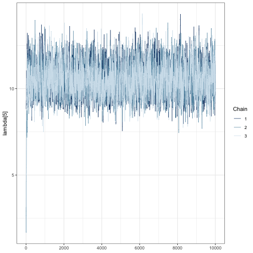

plot of chunk FE_lambda5_trace

We can see that far fewer than 10,000 iterations are likely required because the chains are mixing well after a few hundred iterations. This is shown by strongly overlapping chains, with no one chain appearing by itself in a region of the parameter space. Chains also appear to be stationary because they do not wander vertically substantially after the first few hundred iterations.

We need to check that chains are stationary and mixing for all parameters. One way to accelerate visual inspection this is through the regex_pars argument, which shows relative activity parameters for all species as in the following three code blocks.

mcmc_trace(fit, regex_pars = "lambda")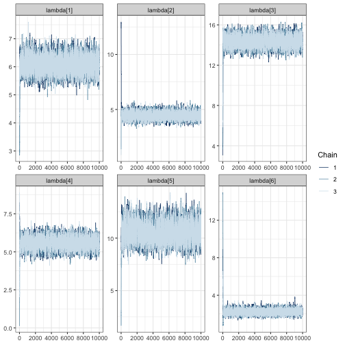

plot of chunk FE_allLambda_trace

mcmc_trace(fit, regex_pars = "psi")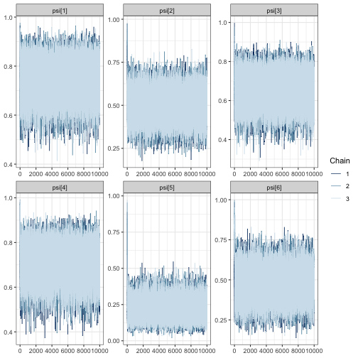

plot of chunk FE_allPsi_trace

# create a traceplot for all elements of the confusion matrix
mcmc_trace(fit, regex_pars = "theta")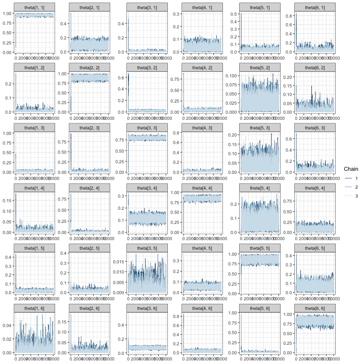

plot of chunk FE_allTheta_trace

In all of the trace plots for all of the parameters, chains appear to mix quickly, meaning that it is possible a far smaller number of iterations may be suitable for a simulation study. A good place to start for reducing the number of iterations is from the output given by tune_mcmc. In our case, we can see that a guess for the minimum number of iterations is 1500 with a warmup of 500:

tune_list$min_iter

## [1] 1500

tune_list$min_warmup

## [1] 500

It is possible to use these values to zoom in on the trace plots by using the window argument:

mcmc_trace(fit, regex_pars = "lambda", window = c(0, tune_list$min_iter))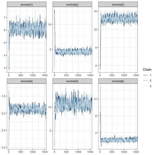

plot of chunk FE_lambdaWindow_trace

Once again, we see the three chains overlap strongly after around 500 iterations and sample around a horizontal line.

After making traceplots and zooming in for all parameters (not all plots are shown here), it appears that the guessed warmup value of 500 output from tune_mcmc is a reasonable choice. Even so, we increase our iterations and warmup beyond the minimum values identified during MCMC tuning to avoid simulations failing due to convergence.

Examine effective sample size and Gelman-Rubin statistics

As a final step, we examine the effective sample sizes (out of 10,000 draws) and $\hat{R}$ values. The effective sample size statistics ess_bulk and ess_tail are MCMC diagnostic statistics that summarizes the number of effectively independent draws from a parameter’s posterior distribution the Markov chain contains. If a parameter has a large value in the ess_bulk column, then it is likely that inference based on sampled draws will characterize the center of the posterior distribution well. The ess_tail column, on the other hand, describes how much information is available about posterior tail probabilities. Once again, we want a large value for ess_tail, preferably ess_tail $\geq 250$ .

tune_list$MCMC_diagnostics

##      parameter   ess_bulk   ess_tail      Rhat
## 1    lambda[1]  4218.6667  5297.4088 1.0010423
## 2    lambda[2]  4076.0509  5140.8523 1.0014264
## 3    lambda[3]  2897.8646  4616.7308 1.0014421
## 4    lambda[4]  2367.5596  4125.9465 1.0013321
## 5    lambda[5]  2560.3580  3366.4861 1.0011913
## 6    lambda[6]  3772.6004  5212.6723 1.0006116
## 7       psi[1] 27151.8325 25478.8872 1.0000906
## 8       psi[2] 29682.1333 29385.7919 1.0000489
## 9       psi[3] 30370.2246 29446.2654 0.9999706
## 10      psi[4] 21960.3976 23857.5083 1.0000184
## 11      psi[5] 17218.4005 10876.1165 0.9999967
## 12      psi[6]  9505.6696 10898.5043 1.0000326
## 13 theta[1, 1]  2261.2405  3894.8878 1.0015458
## 14 theta[2, 1]  3448.0706  3091.8774 1.0018883
## 15 theta[3, 1]  1420.2503  2830.4960 1.0023667
## 16 theta[4, 1]   706.3108   455.0007 1.0034833
## 17 theta[5, 1]  1221.0331  2092.6765 1.0023858
## 18 theta[6, 1]  2732.8527  2502.2704 1.0014545
## 19 theta[1, 2]  2644.2308  3548.7343 1.0011383
## 20 theta[2, 2]  3806.3831  5561.4396 1.0004070
## 21 theta[3, 2]  2599.7503  3486.9707 1.0012877
## 22 theta[4, 2]  2989.1630  4032.9984 1.0014633
## 23 theta[5, 2]  4450.6750  5514.5811 1.0014263
## 24 theta[6, 2]  2894.0111  3048.7690 1.0005577
## 25 theta[1, 3]  1223.9552   854.6336 1.0013618
## 26 theta[2, 3]  1800.6271  2964.3943 1.0008773
## 27 theta[3, 3]  3265.8080  6512.5322 1.0011518
## 28 theta[4, 3]  1548.9196  2213.3120 1.0017995
## 29 theta[5, 3]  1681.3371   937.6103 1.0014029
## 30 theta[6, 3]  1129.7754   842.3393 1.0025348
## 31 theta[1, 4]  3120.6232  3488.6429 1.0010351
## 32 theta[2, 4]  3374.3920  3740.9239 1.0011208
## 33 theta[3, 4]  2986.3822  5560.1731 1.0010900
## 34 theta[4, 4]  2294.7094  5084.9649 1.0017780
## 35 theta[5, 4]  2100.6535  3367.0757 1.0021114
## 36 theta[6, 4]  5383.7712  6184.3521 1.0002718
## 37 theta[1, 5]  4430.5887  6748.9207 1.0010588
## 38 theta[2, 5]  2247.2108  2512.9077 1.0019713
## 39 theta[3, 5]  2899.2511  2937.8658 1.0005982
## 40 theta[4, 5]  5547.5156  6947.6156 1.0004042
## 41 theta[5, 5]  2562.6601  5102.4694 1.0014888
## 42 theta[6, 5]  5084.0200  5131.3701 1.0006520
## 43 theta[1, 6]  3708.0213  4129.4246 1.0009075
## 44 theta[2, 6]  3094.9584  2116.7902 1.0007877
## 45 theta[3, 6]  3169.0384  4637.1122 1.0007562
## 46 theta[4, 6]  4157.8234  6798.1207 1.0006590
## 47 theta[5, 6]  3362.0493  3778.7296 1.0009618
## 48 theta[6, 6]  3573.6909  5807.8722 1.0013958

For all parameters, the bulk and tail effective sample sizes are fairly large, meaning that even with fewer than 10,000 draws, we could expect $n_\text{eff} \geq 250,$ allowing us to characterize both the center and tails of the posteriors for all parameters with these draws. Furthermore, the $\hat{R}$ values for all parameters is near 1. In general, we want values of $\hat{R} \leq 1.1$ for chains to be considered converged. We can double check by recomputing these statistics on shortened chains:

# for each chain, extract iterations 1001:2500 for all parameters
shortened <- lapply(fit, function(x) x[1001:2500,])

# summarize the shortened chains and select the effective sample 
# size columns. mcmc_sum is an internal function used inside of `run_sims`, but
# we use it here to quickly obtain MCMC diagnostics for each parameter
mcmc_sum(shortened, truth = rep(0, ncol(shortened[[1]]))) %>%
  select(parameter, ess_bulk, ess_tail, Rhat)

##      parameter  ess_bulk   ess_tail      Rhat
## 1    lambda[1]  659.6607 1041.47501 1.0124821
## 2    lambda[2]  633.9982  997.64296 1.0124214
## 3    lambda[3]  406.0336  608.21438 1.0041698
## 4    lambda[4]  394.0898  578.31986 1.0057925
## 5    lambda[5]  427.6380  610.52283 1.0043507
## 6    lambda[6]  511.5878  751.58933 1.0068824
## 7       psi[1] 4456.0579 4068.10577 1.0002667
## 8       psi[2] 4695.7869 4341.01096 1.0004376
## 9       psi[3] 4672.3675 4534.57370 1.0000335
## 10      psi[4] 4348.9673 3692.22809 1.0001152
## 11      psi[5] 4277.0253 4397.37233 0.9999471
## 12      psi[6] 1900.6753 3122.80876 0.9998945
## 13 theta[1, 1]  213.2168  510.99337 1.0340076
## 14 theta[2, 1]  420.1724  462.64402 1.0119123
## 15 theta[3, 1]  307.4904  517.58534 1.0017329
## 16 theta[4, 1]  103.1163   78.27652 1.0141918
## 17 theta[5, 1]  202.1417  421.30606 1.0105202
## 18 theta[6, 1]  439.7143  429.26904 1.0028077
## 19 theta[1, 2]  464.6700  477.06672 1.0059255
## 20 theta[2, 2]  461.1501  532.77806 1.0197988
## 21 theta[3, 2]  463.3106  664.46717 1.0041033
## 22 theta[4, 2]  507.0798  605.35790 1.0015923
## 23 theta[5, 2]  707.8389  722.05046 1.0020642
## 24 theta[6, 2]  488.7802  494.06831 1.0040917
## 25 theta[1, 3]  142.3550  107.30974 1.0356507
## 26 theta[2, 3]  271.0448  482.72129 1.0143076
## 27 theta[3, 3]  406.8266  709.78466 1.0048462
## 28 theta[4, 3]  217.6903  461.70333 1.0140200
## 29 theta[5, 3]  199.7939  131.28337 1.0128732
## 30 theta[6, 3]  197.1181  476.37445 1.0356033
## 31 theta[1, 4]  572.7451  648.97553 1.0023786
## 32 theta[2, 4]  515.4881  612.46064 1.0008741
## 33 theta[3, 4]  387.5806  646.46193 1.0037215
## 34 theta[4, 4]  400.0485 1166.26621 1.0057387
## 35 theta[5, 4]  395.7617  741.95632 1.0029655
## 36 theta[6, 4]  897.0067  923.17934 1.0014781
## 37 theta[1, 5]  843.7151 1211.57740 1.0041260
## 38 theta[2, 5]  301.9877  189.22536 1.0191240
## 39 theta[3, 5]  524.2877  570.11696 1.0051693
## 40 theta[4, 5]  838.0160 1194.20555 1.0034813
## 41 theta[5, 5]  427.5636  577.69792 1.0058667
## 42 theta[6, 5]  889.2320  951.93777 1.0032789
## 43 theta[1, 6]  615.6654  842.07190 1.0061096
## 44 theta[2, 6]  639.8041  658.95174 1.0033202
## 45 theta[3, 6]  595.5986  892.41959 1.0014614
## 46 theta[4, 6]  693.8311 1114.37774 1.0032674
## 47 theta[5, 6]  529.0577  529.81216 1.0034092
## 48 theta[6, 6]  687.9854 1489.58173 1.0105002

These results appear satisfactory, with effective sample sizes in both the tail and bulk of the posterior distributions of more than 250 and $\hat{R}$ near 1. Based on the results of MCMC tuning, it appears that using an MCMC with at least 1500 iterations with at least 500 discarded as warmup should to produce good results for our simulation study.

Set iterations for simulation

Based on our findings in the MCMC tuning step, we set the number of iterations for simulation to be slightly higher to guard against convergence issues that preclude using a fitted model for inference:

# to be used in the following section 
iters_for_sims <- tune_list$min_iter + 1000
warmup_for_sims <- tune_list$min_warmup + 500

A note about non-convergence while tuning

In some instances, we have run tune_mcmc with a dataset and received a series of error messages that convergence was not reached in under 10,000 iterations. If this persists after trying to fit several other datasets, we have several options:

We could increase the number of iterations in the simulation study to be above 10,000 – perhaps to 20,000 and settle for a longer run time of the simulation study.
We could take this as a sign that the level of effort is insufficient to identify model parameters. In this case, this scenario should not be considered.

In our experience fitting these models, the second option seems to often be the case, and we encourage users to remove scenarios from consideration if models fit during the tuning step do not reach convergence within 10,000 iterations. It is possible that all validation scenarios – including ones with very large levels of validation effort – will lead to a lack of convergence if the number of sites and visits are very low, in which case the number of sites and visits should be re-evaluated.

We emphasize that the results from tune_mcmc are from a single model fit; they are supplied only as guidelines, and we encourage users to increase the number of iterations above the minimum values output from tune_mcmc. While each model fit will take slightly longer with an increased number of total iterations, this approach may save time in the long run by avoiding the need to re-run simulations.

Step 4: Fit models to simulated data

With the simulated dataset and some informed choices about tuning of the MCMC, we use run_sims to run the simulations:

sims_output <- run_sims(
         data_list = sim_data$masked_dfs, 
         zeros_list = sim_data$zeros, 
         DGVs = list(lambda = lambda, psi = psi, theta = Theta), 
         theta_scenario_id = "FE", # for "fixed effort"
         parallel = TRUE, 
         niter = iters_for_sims, 
         nburn = warmup_for_sims,  
         thin = 1,
         save_fits = TRUE, 
         save_individual_summaries_list = FALSE, 
         directory = tempdir() 
)

The output object, sims_output is a dataframe with summaries of the MCMC draws for each parameter estimated from each dataset under each validation scenario. Summaries include the posterior mean, standard deviation, Naive standard error, Time-series standard error, quantiles for 50% and 95% posterior intervals, median, and MCMC diagnostics (Gelman-Rubin statistic, and effective samples sizes in the tails and bulk of the distribution).

str(sims_output)

## 'data.frame':    1920 obs. of  19 variables:
##  $ parameter     : chr  "lambda[1]" "lambda[2]" "lambda[3]" "lambda[4]" ...
##  $ Mean          : num  6.05 4.8 14.05 5.99 11.81 ...
##  $ SD            : num  0.356 0.345 0.448 0.485 0.801 ...
##  $ Naive SE      : num  0.0053 0.00515 0.00667 0.00723 0.01194 ...
##  $ Time-series SE: num  0.0141 0.0153 0.0175 0.0261 0.0295 ...
##  $ 2.5%          : num  5.38 4.18 13.16 5.03 10.26 ...
##  $ 25%           : num  5.8 4.57 13.76 5.66 11.29 ...
##  $ 50%           : num  6.03 4.79 14.04 6 11.79 ...
##  $ 75%           : num  6.28 5.01 14.33 6.32 12.32 ...
##  $ 97.5%         : num  6.77 5.56 14.97 6.92 13.42 ...
##  $ Rhat          : num  1 1.01 1.01 1.01 1.01 ...
##  $ ess_bulk      : num  643 539 520 269 621 ...
##  $ ess_tail      : num  720 687 874 545 703 ...
##  $ truth         : num  5.93 4.16 14.25 6.2 11.86 ...
##  $ capture       : num  1 0 1 1 1 1 1 1 1 1 ...
##  $ converge      : num  1 1 1 1 1 1 1 1 1 1 ...
##  $ theta_scenario: chr  "FE" "FE" "FE" "FE" ...
##  $ scenario      : int  1 1 1 1 1 1 1 1 1 1 ...
##  $ dataset       : int  1 1 1 1 1 1 1 1 1 1 ...

Note that we fit all models in parallel to reduce simulation time; we encourage users to do the same. However, if you fit models with parallel = FALSE in run_sims, the console will display the messages NIMBLE prints as it compiles code for each model. Internally, we specify a custom distribution to compute the marginal probabilities for ambiguous autoID labels, and you will see a warning about overwriting a custom user-specified distribution if parallel = FALSE. These warnings can be safely ignored.

Step 5: Visualize simulations

Once models have been fit to all simulated datasets, you can visualize results using several functions. We recommend beginning with the most detailed functions, which are visualize_parameter_group and visualize_single_parameter. The plots output from these functions show many following features of the simulation study. These are

Facet grids: parameters (only for visualize_parameter_group)
X-axis: Manual verification scenario
y-axis: parameter values
Small grey error bars: 95% posterior interval for an individual model fit where all parameters were below convergence_threshold.
Colored error bars: average 95% posterior interval across all converged models under that scenario.
Color: Coverage, or the rate at which 95% posterior intervals contain the true data-generating parameter value.
Black points: the true value of the parameter
Red points: average posterior mean

The visualize_parameter_group function is useful for examining an entire set of parameters, such as all relative activity parameters. For example, we can visualize the inference for the relative activity parameters in the first three scenarios in our simulation study above by running the code below.

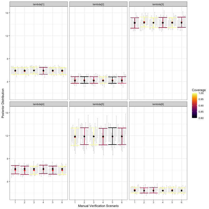
visualize_parameter_group(
  sim_summary = sims_output, 
  pars = "lambda", 
  theta_scenario = 1, 
  scenarios = 1:4,
  convergence_threshold = 1.05
)

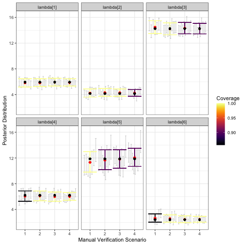
Example output from the visualize_parameter_group function. Results are faceted by parameter, with the x-axis indicating the validation scenario number, and the y-axis showing the data generating value (black point). Red points show average posterior means, small grey intervals show 95% posterior intervals from converged model fits and colored intervals are average 95% posterior intervals. Coverage is shown by color, with blue corresponding to low coverage.

The output figure indicates that under all validation scenarios we considered, the expected inference for relative activity rates of species 1-4 and 6 meets our measurable objectives: the posterior interval width is less than three for these species and there is minimal estimation error. However, note that under validation scenario 1 and 2, fewer of the models converged within 2500 iterations of the MCMC, which is visible from smaller number of grey intervals. This suggests that a higher level of validation effort could be beneficial. Additionally, average interval width is never below 3 for species 5; none of the designs considered here meet the measurable objective for this species. We can see this more clearly by examining output through alternative visualization functions.

A first step would be to use visualize_single_parameter, which takes the same arguments as the previous visualization function:

visualize_single_parameter(
  sims_output, par = "lambda[5]", 
  theta_scenario = 1, 
  scenarios = 1:4, 
  convergence_threshold = 1.05
)

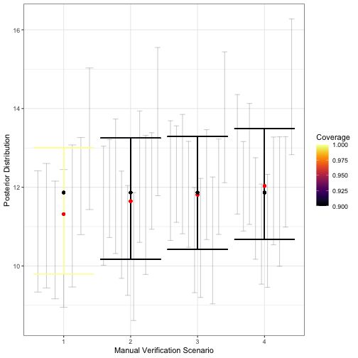
Example output from visualize_single_parameter is similar to that of visualize_parameter_group: the x-axis shows the validation scenario, and the y-axis shows the true value of the parameter (black point). Average posterior means are shown by red points, individual 95% posterior intervals from converged model fits are shown as small grey error bars and average 95% posterior intervals are shown by the larger colored error bars. The coverage is indicated by color.

The greater detail of visualize_single_parameter underscores the difference in the number of converged models, shown by the number grey 95% posterior interval for each converged model fit. The visualization also helps clarify that while average interval width is near 3 in scenario 2, it is still acceptable for our measurable objectives. Coverage for most relative activity parameters is also near-nominal under this validation scenario, which requires that around 375 recordings be validated in an average dataset. This can also be seen using the plot_width_vs_calls function, which compares average interval widths (and the IQR for interval widths) across scenarios based on the number of recordings validated. For example:

# obtain summary of validation effort as an object that can be used with 
# the summary plot functions plot_x_vs_calls
s <-  summarize_n_validated(
  data_list = sim_data$masked_dfs, 
  theta_scenario = "FE", # must not be NULL for the plot_X_vs_calls functions
  scenario_numbers = 1:4
)

plot_width_vs_calls(
  sim_summary = sims_output, 
  calls_summary = s, 
  regex_pars = "lambda", 
  theta_scenario = "FE", 
  scenarios = 2:5
) + # add horizontal line at target 95% CI width 
  geom_hline(yintercept = 3, linetype = "dotted")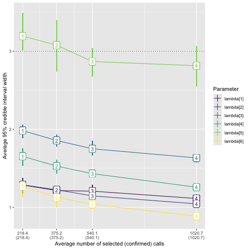

Example output from plot_width_vs_calls. The x-axis shows the number of validated recordings. Note that the level of effort increases with scenario number for the fixed-effort designs; this may not always be the case, for example, with a stratified-by-species design as in the main text. The y-axis shows the value of the average 95% posterior interval width (point). The middle 50% of interval widths for each parameter are shown by the error bars. Color indicates the parameter.

We provide analogous functions plot_coverage_vs_calls and plot_bias_vs_calls taking identical arguments that show how coverage and estimation error change with the number of calls validated. Note that in all of our visualization functions, if no fitted models have $\hat{R} \leq c$ for all parameters, where $c$ is the specified convergence threshold under a given scenario, then the scenario will not appear on the x-axis. In our example, we used $c = 1.1$ .

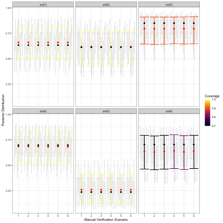
To ensure that there aren’t substantial problems with estimation of other model parameters, we can create plots for $\psi$ and $\Theta$ :

visualize_parameter_group(
  sim_summary = sims_output, 
  pars = "psi", 
  theta_scenario = 1, 
  scenarios = 1:4,
  convergence_threshold = 1.05
)

$We encourage users to check inference for other model parameters, even if they are not explicitly of interest based on measurable objectives. Here, we examine \boldsymbol{\psi}. Note that coverage for several parameters is slightly low. For the purpose of exposition, we only fit 10 datasets and we expect that coverage would be near nominal levels if 50 or more datasets were used in simulation.$

We encourage users to check inference for other model parameters, even if they are not explicitly of interest based on measurable objectives. Here, we examine

\boldsymbol{\psi}

. Note that coverage for several parameters is slightly low. For the purpose of exposition, we only fit 10 datasets and we expect that coverage would be near nominal levels if 50 or more datasets were used in simulation.

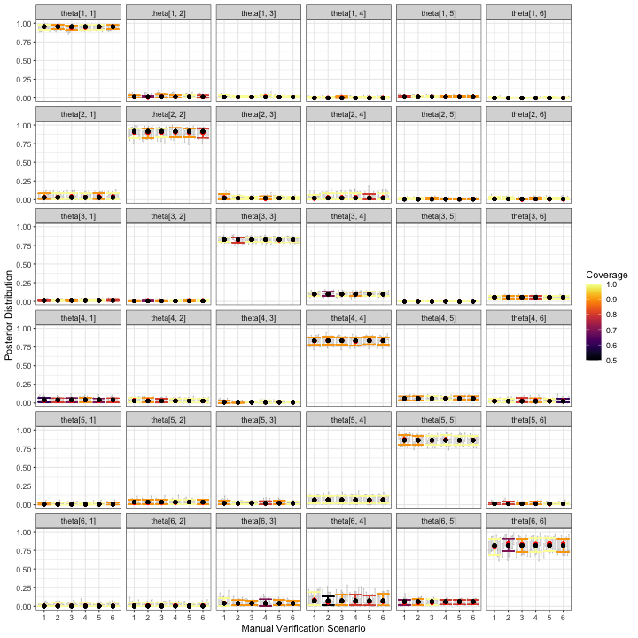
visualize_parameter_group(
  sim_summary = sims_output, 
  pars = "theta", 
  theta_scenario = 1, 
  scenarios = 1:4,
  convergence_threshold = 1.05
)

$Checking inference for the elements of the classification matrix \Theta. For most parameters (facets), validation scenario 2 appears to lead to minimal estimation error and near-nominal coverage.$

Checking inference for the elements of the classification matrix

\Theta

. For most parameters (facets), validation scenario 2 appears to lead to minimal estimation error and near-nominal coverage.

The simulation results for $\boldsymbol{\psi}$ and $\Theta$ don’t immediately cause concern that inference for relative activity rates will be severely compromised for any of these validation designs. Some parameters have slightly low coverage, but we believe this is mostly due to the small number of datasets used in this example; users should increase the number of datasets to at least 50, which we expect would lead to coverage near nominal levels.

Take-aways from the Fixed-Effort Simulations

Based on the simulation results shown in the figures above, we can rule out validation scenario 1, because the expected width of 95% posterior intervals is greater than the threshold value of 3. Because of this, we might choose validation scenario 2 as one possible fixed effort validation design. This fixed effort design assumes that 10% of recordings from each site-night are randomly selected for validation, leading to around 375 recordings being validated per dataset. In our simulations, posterior means for each $\lambda_k$ appear to be nearly unbiased, with near-nominal coverage and average posterior interval widths less than or equal to 3 for this scenario. However, it is possible that for a given dataset, the interval width for $\lambda_5$ will be larger than 3, regardless of the number of validated calls; in the plot of calls versus interval widths, error bars overlap or exceed the dotted line in all scenarios.

In situations such as this one, a decision is required of the user. If a slightly larger interval width is acceptable, validating 10% percent of recordings from all site-visits is reasonable. If it is not, then the LOVE will need to be increased beyond that in scenario 4 (1021 recordings). The question is whether potentially tripling the number of validated recordings will be worth the benefit of ensuring the relative activity level for species 5 is less than 3. This is a question about measurable objectives that we leave to the practitioner and their study priorities.

Stratified-by-species example

In this section, we provide further details of the example in the main manuscript, which assumed a stratified-by-species design. In a stratified-by-species design, the random mechanism is a stratified random sample, with strata formed by the species labels assigned during automated classification (i.e., by autoID). In this type of design, the LOVE is the proportion of recordings selected to be validated for each species label.

We repeat the simulation study conducted in the main text in this section, providing greater detail for some of the steps. We assume the same measurable objectives as in the fixed effort example, but we now assume the maximum number of recordings that can be viewed by experts during the validation process is 1000.

Simulate data

Using the same values for psi, lambda and Theta as in the previous example, we simulate data using simulate_validatedData with design_type = "BySpecies" and set the probability of successfully validating a selected recording using the confirmable_limits argument.

sim_data <- simulate_validatedData(
  n_datasets = 10, 
  design_type = "BySpecies",
  scenarios = list(
    spp1 = 0.15, 
    spp2 = 0.15, 
    spp3 = c(0.15, .5, 1),
    spp4 = 0.1, 
    spp5 = c(0.5, 1),
    spp6 = 0.25
  ),
  nsites = nsites, 
  nspecies = nspecies, 
  nvisits = nvisits,
  psi = psi, 
  lambda = lambda, 
  theta = Theta, 
  directory = tempdir()
)

Note that in contrast with the fixed effort example, simulate_validatedData expects the scenarios argument to be a list of proportions corresponding to the possible levels of effort for each species when specifying a stratified-by-species design. Internally, simulate_validatedData calls base::expand.grid, and considers all possible combinations of the various levels of effort for each species, meaning that the number of simulated scenarios grows extremely quickly. The biggest implication of having a larger number of simulation scenarios to consider is increased computation time. For example, in the previous code block we fixed the level of effort for species 1, 2, 4 and 6 at .15, .15, .1, and .25, respectively. There are three possible proportions to validate for species 3 and two possible levels of effort for species 5, yielding six possible scenarios, which are summarized in the additional output sim_data$scenarios_df that is available when design_type = "BySpecies" is specified:

names(sim_data)

## [1] "full_datasets" "zeros"         "masked_dfs"    "scenarios_df"

sim_data$scenarios_df

##   scenario spp1 spp2 spp3 spp4 spp5 spp6
## 1        1 0.15 0.15 0.15  0.1  0.5 0.25
## 2        2 0.15 0.15 0.50  0.1  0.5 0.25
## 3        3 0.15 0.15 1.00  0.1  0.5 0.25
## 4        4 0.15 0.15 0.15  0.1  1.0 0.25
## 5        5 0.15 0.15 0.50  0.1  1.0 0.25
## 6        6 0.15 0.15 1.00  0.1  1.0 0.25

If users would like to supply a tailored set of validation scenarios, this can be done through the scen_expand and scen_df arguments as follows:

# Define the scenarios dataframe. Each row is a scenario, each column is a spp
my_scenarios <- data.frame(
  spp1 = c(0.05, 0.05, 0.1), 
  spp2 = c(0.1, 0.2, 0.3),
  spp3 = c(0.2, 0.2, 0.25), 
  spp4 = c(0.4, 0.5, 0.6), 
  spp5 = rep(1, 3), 
  spp6 = rep(0.5, 3)
)

sim_data2 <- simulate_validatedData(
  n_datasets = 10, 
  design_type = "BySpecies",
  scen_expand = FALSE, 
  scen_df = my_scenarios,
  scenarios = NULL,
  nsites = nsites, 
  nspecies = nspecies, 
  nvisits = nvisits,
  psi = psi, 
  lambda = lambda, 
  theta = Theta, 
  directory = tempdir()
)

sim_data2$scenarios_df # the same as my_scenarios above

##   scenario spp1 spp2 spp3 spp4 spp5 spp6
## 1        1 0.05  0.1 0.20  0.4    1  0.5
## 2        2 0.05  0.2 0.20  0.5    1  0.5
## 3        3 0.10  0.3 0.25  0.6    1  0.5

In the remainder of this example, we use the sim_data object. We can combine the scenarios_df output with the output of summarize_n_validated to understand what the scenarios are and how many recordings are validated under each.

summary1 <- sim_data$scenarios_df
summary2 <- summarize_n_validated(
  sim_data$masked_dfs, 
  scenario_numbers = 1:6,
  theta_scenario = "BySpecies"
)

call_sum <- left_join(summary1, summary2, by = "scenario")

call_sum

##   scenario spp1 spp2 spp3 spp4 spp5 spp6 theta_scenario n_selected
## 1        1 0.15 0.15 0.15  0.1  0.5 0.25      BySpecies      603.8
## 2        2 0.15 0.15 0.50  0.1  0.5 0.25      BySpecies     1018.3
## 3        3 0.15 0.15 1.00  0.1  0.5 0.25      BySpecies     1610.4
## 4        4 0.15 0.15 0.15  0.1  1.0 0.25      BySpecies      778.3
## 5        5 0.15 0.15 0.50  0.1  1.0 0.25      BySpecies     1192.8
## 6        6 0.15 0.15 1.00  0.1  1.0 0.25      BySpecies     1784.9
##   n_validated
## 1       603.8
## 2      1018.3
## 3      1610.4
## 4       778.3
## 5      1192.8
## 6      1784.9

In the resulting dataframe, we see that scenario 1 has the lowest overall level of validation effort: species 1-3 have 15% of their recordings validated, species 4 has 10% validated, species 5 has 50%, and species 6 has 25%, yielding around 604 recordings validated in an average dataset. We use one dataset simulated under scenario 1 to tune the MCMC.

Tune the MCMC

The MCMC tuning in this step is very similar to the procedures used to tune the MCMC in the fixed effort example. We begin by fitting a model to one dataset using the tune_mcmc function.

i <- sample(1:length(sim_data$full_datasets), 1)

tune_list <- tune_mcmc(
  dataset = sim_data$masked_dfs[[1]][[i]],
  zeros = sim_data$zeros[[i]]
)

## [1] "Fitting MCMC in parallel ... this may take a few minutes"

We visually inspect the chains for convergence using trace plots. We set trace plot windows to be wider than the suggested values from tune_mcmc, meaning a lower starting value and a higher ending value. Based on these plots, chains appear to be mixing well as no one chain stands out visually.

tune_list$min_warmup

## [1] 500

tune_list$min_iter

## [1] 1500

# increase iters to visualize beyond the warmup and 
# iterations output from tune_mcmc 
fit <- tune_list$fit

mcmc_trace(fit, regex_pars = "lambda", window = c(0, tune_list$min_iter + 500))

plot of chunk BSV_lambdaWindow_trace

mcmc_trace(fit, regex_pars = "psi", window = c(0, tune_list$min_iter + 500))

plot of chunk BSV_psiWindow_trace

mcmc_trace(fit, regex_pars = "theta", window = c(0, tune_list$min_iter + 500))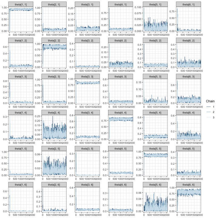

plot of chunk BSV_thetaWindow_trace

In all trace plots, it appears that MCMC chains have reached approximate convergence well before the warmup value of 500 draws output from tune_mcmc.

Next, we examine the effective sample sizes in the tails and bulk of the posteriors and the $\hat{R}$ values:

tune_list$MCMC_diagnostics

##      parameter  ess_bulk  ess_tail      Rhat
## 1    lambda[1]  4785.187  6015.156 1.0002953
## 2    lambda[2]  3482.169  4671.583 1.0010385
## 3    lambda[3]  4010.305  5077.642 1.0011804
## 4    lambda[4]  3838.985  5066.782 1.0005667
## 5    lambda[5]  4389.305  6076.436 1.0005144
## 6    lambda[6]  3406.792  4158.077 1.0004562
## 7       psi[1] 29121.024 23900.572 1.0000143
## 8       psi[2] 29804.548 28990.720 0.9999733
## 9       psi[3] 30171.029 28065.621 0.9999970
## 10      psi[4] 29714.743 30187.849 0.9999654
## 11      psi[5] 26941.892 27878.460 1.0000525
## 12      psi[6] 22975.041 24021.093 1.0000437
## 13 theta[1, 1]  5787.766  9100.303 1.0004077
## 14 theta[2, 1]  3455.126  3155.152 1.0006055
## 15 theta[3, 1]  4497.881  6507.510 1.0008888
## 16 theta[4, 1]  5448.294  7671.854 1.0004599
## 17 theta[5, 1]  4422.335  4442.610 1.0007224
## 18 theta[6, 1]  3346.556  3904.648 1.0003512
## 19 theta[1, 2]  4197.079  6509.295 1.0000984
## 20 theta[2, 2]  4671.424  6916.745 1.0002588
## 21 theta[3, 2]  4977.624  6018.970 1.0002021
## 22 theta[4, 2]  3768.818  4339.586 1.0006414
## 23 theta[5, 2]  5832.809  7764.025 1.0006486
## 24 theta[6, 2]  3972.024  4916.645 1.0003475
## 25 theta[1, 3]  4106.142  5400.044 1.0003499
## 26 theta[2, 3]  4255.177  4675.944 1.0006575
## 27 theta[3, 3]  4864.204  8569.148 1.0014585
## 28 theta[4, 3]  4559.116  5859.463 1.0004257
## 29 theta[5, 3]  2354.970  2196.293 1.0022593
## 30 theta[6, 3]  3726.412  5771.138 1.0006064
## 31 theta[1, 4]  2855.605  2506.061 1.0008671
## 32 theta[2, 4]  3964.252  6380.398 1.0011764
## 33 theta[3, 4]  3864.012  6188.563 1.0012619
## 34 theta[4, 4]  6352.542  9022.962 1.0003353
## 35 theta[5, 4]  4401.833  6435.479 1.0005240
## 36 theta[6, 4]  4056.456  5345.106 1.0009939
## 37 theta[1, 5]  8474.764 11130.448 1.0004465
## 38 theta[2, 5]  6236.015  7361.206 1.0004429
## 39 theta[3, 5]  2798.787  3910.813 1.0014421
## 40 theta[4, 5]  6898.849  8812.403 1.0004727
## 41 theta[5, 5]  5311.251  9890.303 1.0002080
## 42 theta[6, 5]  5837.553  7243.298 1.0006446
## 43 theta[1, 6]  3392.526  4186.108 1.0019124
## 44 theta[2, 6]  2456.909  1244.644 1.0008431
## 45 theta[3, 6]  4282.198  3193.990 1.0014370
## 46 theta[4, 6]  4898.688  4414.135 1.0016046
## 47 theta[5, 6]  4864.306  5687.563 1.0016675
## 48 theta[6, 6]  4556.444  7105.185 1.0001742

For all parameters, the bulk and tail effective sample sizes are fairly large: if we slightly decrease the number of post-warmup draws, we could expect to characterize both the center and tails of the posteriors well. Additionally, $\hat{R} \approx 1.00$ for all parameters, indicating good mixing for chains. As before, we check this suspicion by computing MCMC diagnostic statistics for truncated chains:

# for each chain, extract iterations 501:2000 for all parameters
shortened <- lapply(fit, function(x) x[(tune_list$min_warmup):tune_list$min_iter + 1000,])

# summarize the shortened chains and select the effective sample 
# size columns
mcmc_sum(shortened, truth = rep(0, ncol(shortened[[1]]))) %>%
  select(parameter, ess_bulk, ess_tail)

##      parameter  ess_bulk  ess_tail
## 1    lambda[1]  574.1892  633.6262
## 2    lambda[2]  348.2909  614.8738
## 3    lambda[3]  435.9153  589.8075
## 4    lambda[4]  382.8387  499.1073
## 5    lambda[5]  459.0001  612.6886
## 6    lambda[6]  442.3031  621.4838
## 7       psi[1] 3048.3363 2970.2396
## 8       psi[2] 3156.8813 2939.1626
## 9       psi[3] 3105.5931 2634.2629
## 10      psi[4] 2771.7190 2886.5934
## 11      psi[5] 2724.5111 2710.7067
## 12      psi[6] 2765.9277 2868.8254
## 13 theta[1, 1]  718.2535 1118.7205
## 14 theta[2, 1]  507.1318  816.7757
## 15 theta[3, 1]  532.8965  607.5688
## 16 theta[4, 1]  676.0604  945.1029
## 17 theta[5, 1]  474.9767  493.7329
## 18 theta[6, 1]  331.1427  328.2412
## 19 theta[1, 2]  378.4661  542.1534
## 20 theta[2, 2]  461.7568  867.3559
## 21 theta[3, 2]  582.5390  712.0605
## 22 theta[4, 2]  419.8620  512.9908
## 23 theta[5, 2]  635.0468  895.2092
## 24 theta[6, 2]  468.9389  648.5659
## 25 theta[1, 3]  464.9002  631.3908
## 26 theta[2, 3]  464.9974  579.8377
## 27 theta[3, 3]  475.3561 1075.7107
## 28 theta[4, 3]  522.3379  734.1960
## 29 theta[5, 3]  390.0819  433.5848
## 30 theta[6, 3]  494.3521  818.0141
## 31 theta[1, 4]  338.1179  302.2860
## 32 theta[2, 4]  352.6493  580.8035
## 33 theta[3, 4]  357.5814  668.1405
## 34 theta[4, 4]  864.2150 1367.6856
## 35 theta[5, 4]  498.6143  726.9613
## 36 theta[6, 4]  479.4368  719.9665
## 37 theta[1, 5]  823.2224  993.5574
## 38 theta[2, 5]  592.2021  681.8409
## 39 theta[3, 5]  330.7999  264.4705
## 40 theta[4, 5]  854.1993  895.0335
## 41 theta[5, 5]  528.4875 1040.5071
## 42 theta[6, 5]  665.5349  656.5485
## 43 theta[1, 6]  451.3428  478.1981
## 44 theta[2, 6]  375.2597  397.9304
## 45 theta[3, 6]  563.7432  948.9868
## 46 theta[4, 6]  583.7598  665.7532
## 47 theta[5, 6]  544.3184  705.7296
## 48 theta[6, 6]  563.8011 1075.2020

The results appear satisfactory, with effective sample sizes of more than 250 in both the tail and bulk of the posterior distributions for each parameter. Based on the results of MCMC exploration, it appears that using an MCMC with 2500 iterations with 500 discarded as warmup is likely to produce good results for our simulation study.

Fit models

sims_out <- run_sims(
  data_list = sim_data$masked_dfs,
  zeros_list = sim_data$zeros,
  DGVs = list(lambda = lambda, psi = psi, theta = Theta),
  theta_scenario_id = "BySpecies", 
  parallel = TRUE,
  niter = tune_list$min_iter + 500, 
  nburn = tune_list$min_warmup + 250,
  thin = 1, 
  save_fits = FALSE,
  save_individual_summaries_list = FALSE,
  directory = tempdir()
)

The output, sims_out, will have the same structure as in the fixed effort example.

Visualize results

Recall that the measurable objectives of our study are to estimate the relative activity rates with estimation error less than 1 call per night and a 95% posterior interval width of less than 3 calls per night. Furthermore, we assume that the monitoring program can afford to validate 4000 calls in total. All of the possible validation designs shown in sim_data$scenarios_df are feasible given this budget.

We begin with detailed plots of relative activity rates, occurrence probabilities, and classification probabilities.

visualize_parameter_group(
  sim_summary = sims_out, 
  pars = "lambda",
  theta_scenario = "BySpecies", 
  scenarios = 1:6, 
)

Output from visualize_parameter_group under six possible stratified-by-species scenarios for relative activity rates. Parameters are shown in each facet and validation scenario number is on the x-axis. Small grey intervals are 95% posterior intervals for each parameter from fitted models that converged. Larger colored error bars are average 95% posterior intervals with the color indicating the coverage. Black dots are the true parameter value and red dots are average posterior means.

Based on the simulation results for $\boldsymbol{\lambda}$ , any of validation scenarios 1-6 is expected to produce a posterior mean estimate for each relative activity parameter that is near the true value. All models converged for all scenarios. Coverage varies by scenario for each parameter, but recall that we only fit models to 10 datasets.

visualize_parameter_group(
  sim_summary = sims_out, 
  pars = "psi",
  theta_scenario = "BySpecies", 
  scenarios = 1:6, 
)

Output from visualize_parameter_group under six possible stratified-by-species scenarios for occurrence probabilities. Parameters are shown in each facet and validation scenario number is on the x-axis. Small grey intervals are 95% posterior intervals for each parameter from fitted models that converged. Larger colored error bars are average 95% posterior intervals with the color indicating the coverage. Black dots are the true parameter value and red dots are average posterior means.

The simulation results for occurrence probabilities show a small amount estimation error for all occurrence probabilities, with the size and direction varying depending on the species. For species with larger estimation error, coverage is also slightly low. However, since we are most concerned with relative activity, the goal is to check results for each $\psi_k$ for severe estimation error and/or lack of coverage, which are not shown in the figure above. Similarly, we do not observe alarming simulation results for $\Theta$ :

visualize_parameter_group(
  sim_summary = sims_out, 
  pars = "theta",
  theta_scenario = "BySpecies", 
  scenarios = 1:6, 
)

Output from visualize_parameter_group under six possible stratified-by-species scenarios for classification probabilities. Parameters are shown in each facet and validation scenario number is on the x-axis. Small grey intervals are 95% posterior intervals for each parameter from fitted models that converged. Larger colored error bars are average 95% posterior intervals with the color indicating the coverage. Black dots are the true parameter value and red dots are average posterior means.

One measurable objective is for 95% posterior interval widths to be less than 3 calls per night for each species’ relative activity rate. The plot_width_vs_calls function addresses this measurable objective directly:

plot_width_vs_calls(
  sim_summary = sims_out, 
  calls_summary = call_sum, 
  regex_pars = "lambda",
  theta_scenario = unique(sims_out$theta_scenario),
  scenarios = 1:6,
  max_calls = 1000 # put shading over scenarios that are beyond budget
)

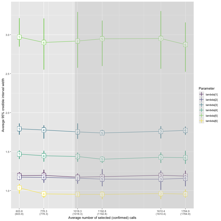
Plots of 95% posterior interval width vs the number of calls validated.

As observed previously, the widest posterior interval width is for species 5. All validation scenarios have average 95% posterior interval widths near or slightly below 3 calls per night, but the error bars indicate an interval width greater than 3 is possible for any validation scenario. Scenario 6, in which 1785 recordings are validated, has the narrowest expected interval width.

Take-aways

The simulation results for by-species validation imply that, of the stratified-by-species validation designs considered, scenario 6 offered the best results with respect to the measurable objectives. In this scenario, the six species in our assemblage receive 15%, 15%, 100%, 10%, 100%, and 25% of their recordings validated, respectively.

To keep the number of scenarios in this example small, we fixed the LOVE for several species. However, if the measurable objectives specified the desired accuracy and precision for estimates of occurrence probability, it may be desirable to consider alternative validation scenarios. For example, we consistently underestimated the occurrence probability for species 6 (see plot of average posterior means and average 95% credible intervals for each $\psi_k$ ), and additional simulations under validation designs that varied the level of effort for species 6 would be warranted if measurable objectives related to occurrence probability for this species.

Conclusion

We have demonstrated the use of the ValidationExplorer package when the objective is to compare the merits of four competing LOVEs for fixed-effort and stratified-by-species designs. Specifically, in the fixed-effort design we considered validating a random sample of 5%, 10%, 15% or 30% of the recordings obtained during each visit to each site. In the stratified-by-species designs, we considered a suite of validation designs, fixing effort for species 1,2, 4, and 6 at less than or equal to 25%, and varied the level of effort for species 3 and 5. The exact simulations considered are summarized in the call_sum object in Section @ref(simBySpp). The measurable objectives were to estimate the relative activity parameters for each species, with near-nominal coverage and width less than 3 calls per night for 95% posterior intervals. Results, and their implications for these measurable objectives were summarized at the end of each example. Practitioners who would like to inform study design prior to data collection can repeat multiple simulation studies to see how inferences change with the number of sites and balanced visits, in addition to the validation design.

References

Gabry, Jonah, Daniel Simpson, Aki Vehtari, Michael Betancourt, and Andrew Gelman. 2019. “Visualization in Bayesian Workflow.” J. R. Stat. Soc. A 182: 389–402. https://doi.org/10.1111/rssa.12378.

Loeb, Susan C., Thomas J. Rodhouse, Laura E. Ellison, Cori L. Lausen, Jonathan D. Reichard, Kathryn M. Irvine, Thomas E. Ingersoll, et al. 2015. “A Plan for the North American Bat Monitoring Program (NABat).” SRS-208. USDA Forest Service.

Stratton, Christian, Kathryn M. Irvine, Katharine M. Banner, Wilson J. Wright, Cori Lausen, and Jason Rae. 2022. “Coupling Validation Effort with in Situ Bioacoustic Data Improves Estimating Relative Activity and Occupancy for Multiple Species with Cross-Species Misclassifications.” Methods in Ecology and Evolution 13 (6): 1288–1303. https://doi.org/https://doi.org/10.1111/2041-210X.13831.

2026-04-02